Binning the Voltage Values
First I plotted a histogram of a random sampling of 0.1% of these points to get an idea of whether they were equally distributed in voltage space or not. Surprisingly, there are sharp peaks throughout the voltage rather than an equal distribution.
In this graph, the x axis is voltage and the y axis is the number of points found at each voltage.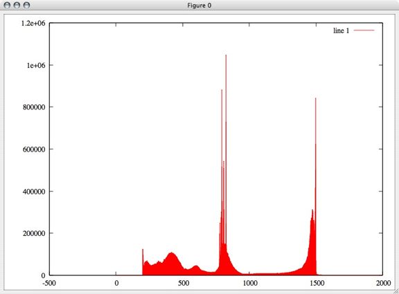
Next I performed kmeans clustering on the points to create bins for the voltage values. This allowed me to come up with a discritization of the voltage values. For simplicity's sake, I started with a relatively small number of bins. I decided to use 6 bins for the voltage values.
This image is of FIVE bins, not 6. I'll be putting up the real image soon, but to give an idea this graph is a dummy value on the x value for plotting purposes, and the voltage points are plotted on the y axis colored according to the cluster they belong to: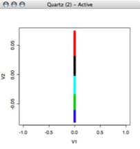 Once the data in my training set was assigned to clusters, I was able to use that data to find the boundaries of the clusters. I wrote a brute force MatLab function that went through each cluster to find the highest and lowest value in each cluster. Column 1 is the number of points in that cluster, column 2 is the minimum value in the cluster, and column 3 is the maximum value.
In Cluster 1:  174158 0.039213 0.073395
In Cluster 2:  32334 0.019467 0.039213
In Cluster 3:  20602 -0.0058785 0.019465
In Cluster 4:  189199 -0.034651 -0.0058841
In Cluster 5:  131339 -0.059631 -0.034652
In Cluster 6:  129368 -0.079999 -0.059631
Discritizing the MinMax plots
Next, I used these values to write a java method that goes through astrid's database and discritizes all of the MinMax Vectors. For example, this model (where the second column is the voltage value for each point):
996018
0.000000e+00 4.974533e-02 1 -4.838973e-02
6.300000e-03 -1.097534e-02 0 -4.823223e-02
1.110000e-02 -9.882242e-03 1 -4.811223e-02
1.026000e-01 -7.579889e-02 0 -4.703479e-02
7.241000e-01 4.974689e-02 1 -4.701274e-02
7.304000e-01 -1.097532e-02 0 -4.685524e-02
7.352000e-01 -9.882236e-03 1 -4.673524e-02
8.267000e-01 -7.579889e-02 0 -4.565805e-02
1.448200e+00 4.974609e-02 1 -4.563577e-02
1.454500e+00 -1.097523e-02 0 -4.547827e-02
1.459300e+00 -9.882241e-03 1 -4.535827e-02
1.550800e+00 -7.579889e-02 0 -4.428133e-02
becomes:
996018 6 3 3 1 6 3 3 1 6 3 3 1
Creating Feature Vectors
Next, I reduced this even further by creating a vector for each model that contains the percentage of its points contained in each voltage bin. This meant that every model was then described by 6 numbers, each one a percentage value so they could be compared to each other.
Thus, the above model became:
0.25 0.00 0.5 0.0 0.0 0.25
Because 25% of it is made up of 1's, 0% of 2's, 50% of 3's, 0% of 4's or 5's and 25% of 6's.
A First Glimpse Through PCA
First I performed principle component analysis on this data to see if it could be reduced even further, but all 6 dimensions turned out to be pretty useful. Even so, after transforming the data based only on the first 3 principal components, we can see some clearly defined separation between groups. My hope is that by using all 6 dimensions, we can get some even clearer distinction and more groups.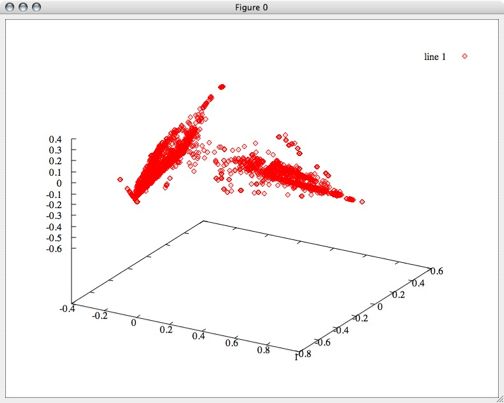
More Detail With kMeans
Next, I performed kmeans clustering on the percentage vectors, using several different numbers of clusters.
4 Clusters: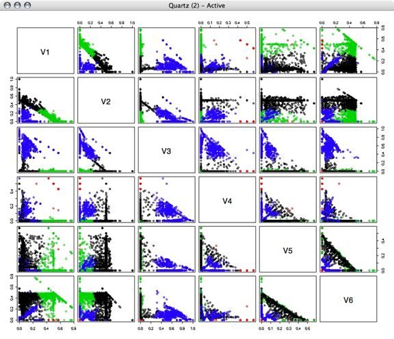 5 Clusters:
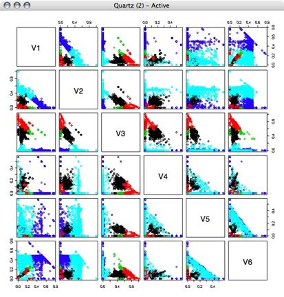 6 Clusters:
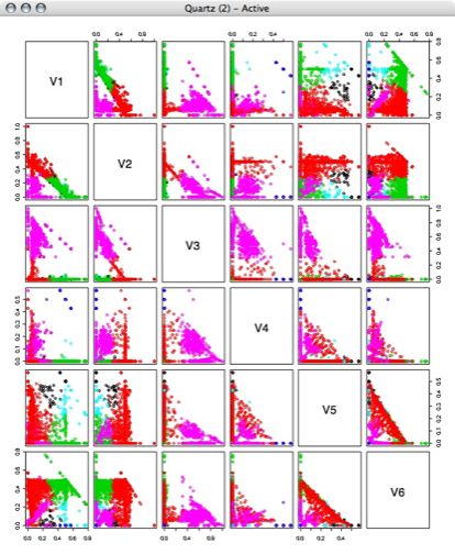 7 Clusters:
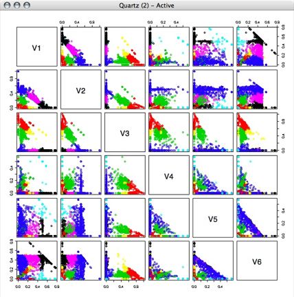
Looking at this now, I think we might be able to get even better classifications by putting the data into a better projection, but I haven't done that yet.
Building Rules to Classify Models
My next step was to choose one of the clustering assignments (I chose the 7 clusters assignments) to find out what defines each cluster. Using a similar technique to the one I used to determine the binning boundaries for voltage (above), I found the boundaries for each cluster for each of the six "features."
For each cluster, the rows indicate the voltage bin, the first column indicates the lowest percentage boundary and the second column indicates the highest percentage boundary for each bin. For a quick pass, I used these to create rule sets to assign labels to the data rather than defining the linear boundaries. This approach was able to assign labels to roughly 80% of the data.
cluster 1:
0.16456  0.50000
0.00000  0.38298
0.00000  0.04167
0.00000  0.03571
0.30000  0.57143
0.00000  0.16667
cluster 2:
0.02273  0.37410
0.25000  1.00000
0.00000  0.18750
0.00000  0.57143
0.16667  0.57143
0.08571  0.57143
Cluster 3:
0.23077  0.76923
0.00000  0.31579
0.00000  0.06250
0.00000  0.05000
0.00000  0.22652
0.22917  0.76923
Cluster 4:
0.25000  0.57143
0.00000  0.00000
0.00000  0.00000
0.42857  0.57143
0.00000  0.00000
0.00000  0.25000
Cluster 5:
0.39550  0.76923
0.00000  0.22186
0.00000  0.03846
0.00000  0.16667
0.15714  0.46154
0.00000  0.25658
Cluster 6:
0.06250  0.57143
0.00000  0.07722
0.31579  0.87500
0.00000  0.10000
0.00000  0.06122
0.12500  0.52632
Cluster 7:
0.03774  0.30769
0.00000  0.57143
0.16364  1.00000
0.00913  0.57143
0.00000  0.33333
0.04110  0.21053
I ran a preliminary classification on the database using these clusters

No comments:
Post a Comment